In December 2010 two friends Philip Vanstraceele and Luc Allaeys finished an interesting research paper they called Systematic Value Investing: Does it really work?
They wanted to find out:
- What was the best investment strategy in Europe over the 11-years from June 1999 to June 2010
- If small companies perform better than large companies
- If 30 stock portfolios do better than 50 stock portfolios
What they found was really interesting and I asked them if I can write it up to share with you here.
Before I tell you exactly what the best strategy was first some information on how and what they tested.
Back test period – 11 years
They did all their testing over the 11-year period from 13 June 1999 to 13 June 2010.
This is not that long but it included the bursting of the internet bubble and the financial crisis so it was a tough investment period.
Back test universe – Eurozone
The back test universe included all the companies listed in the Eurozone excluding banks and insurance companies.
Nine value investing strategies tested
They tested the following nine value investment strategies.
1. The Magic Formula (MF)
This is the very well-known Magic Formula investment strategy from the great book by Joel Greenblatt “The little book that beats the market”.
To find investment ideas for this strategy the investment universe was ranked from high to low by their Return on Invested Capital (ROIC). The company with the highest (best) ROIC gets ranking 1 and the company with the lowest gets the highest value, for example 2000.
Next the universe is ranked the same way by Earning Yield (EY = EBIT/Enterprise Value). The company with the highest (best) EY is ranked 1, and the company with the lowest earning yield receives ranking 2000.
Finally they added these two rankings and sorted all the companies from low to high using this combined ranking.
The Magic Formula looks for companies that have the best combination of both two factors. So a company that is ranked 232 in ROIC and 153 in EY, gets a better combined ranking (232+153=385) than a company that is ranked 1 in ROIC but only 1150 in EY (1+1150= 1151).
2. ERP5
The ERP5 investment strategy looks for companies that are cheap and have earnings power using the following four ratios:
- Earning Yield : (EBIT/Enterprise Value) - How much is a business earning compared to its enterprise value.
- ROIC : Last 12 months (Return On Invested Capital = EBIT / ((Net working capital) + Net Fixed Assets) - ROIC tells you how effectively a company uses it’s invested capital to generate returns
- Price to Book Value - This ratio tells you how cheap a company is compared to its book value.
- Five year trailing ROIC: (Five year average EBIT / Five year average ((Net working capital) + Net Fixed Assets) - This ratio tells you how effectively a company used its invested capital over the past five years. Because of the five year average it helps you screen out a company with a record one year return on invested capital. Steady companies earning a good return on invested capital are selected with this ratio.
The investment universe is ranked the same way using these four ratios the same as the Magic Formula ranking is done.
3. Piotroski 's F-score for low price to book companies (PIOT)
In a research paper published in 2000 Joseph Piotroski, an accounting professor from the University of Chicago, developed and successfully tested a system to improve the returns of a low price to book investment strategy.
He did this with the use of a few simple accounting ratios which he used to develop nine point scoring system.
He found that if you only bought companies that scored highest (8 or 9) on his 9-point scale, or F-Score as he called it, over the 20-year period from 1976 to 1996 you would have out-performed the US market by 13.4% per year on average.
This is also the strategy they tested - a low price to book ratio combined with a high Piotroski F-score.
This is how the Piotroski F-Score is calculated:
Profitability
1. Return on Assets (ROA)
Net income before extraordinary items for the year divided by total assets at the beginning of the year. Score 1 if positive, 0 if negative
2. Cash Flow Return on Assets (CFROA)
Net cash flow from operating activities (operating cash flow) divided by total assets at the beginning of the year.
Score 1 if positive, 0 if negative
3. Change in return on assets
Compare this year’s return on assets (Ratio 1) to last year’s return on assets. Score 1 if it’s higher, 0 if it’s lower
4. Quality of earnings (accrual)
Compare Cash flow return on assets (Ratio 2) to return on assets (Ratio 1) Score 1 if CFROA>ROA, 0 if CFROA<ROA
Funding
5. Change in gearing or leverage
Compare this year’s gearing (long-term debt divided by average total assets) to last year’s gearing. Score 1 if gearing is lower, 0 if it’s higher.
6. Change in working capital (liquidity)
Compare this year’s current ratio (current assets divided by current liabilities) to last year’s current ratio. Score 1 if this year’s current ratio is higher, 0 if it’s lower
7. Change in shares in issue
Compare the number of shares in issue this year, to the number in issue last year.
Score 1 if there are the same or fewer shares in issue this year. Score 0 if there are more shares in issue.
Efficiency
8. Change in gross margin
Compare this year’s gross margin (gross profit divided by sales) to last year’s. Score 1 if this year’s gross margin is higher, 0 if it’s lower
9. Change in asset turnover
Compare this year’s asset turnover (total sales divided by total assets at the beginning of the year) to last year’s asset turnover ratio.
Score 1 if this year’s asset turnover ratio is higher, 0 if it’s lower
Evaluation
Piotroski or F-Score = 1 + 2 + 3 + 4 + 5 + 6 + 7 + 8 + 9 Good or high score = 8 or 9
Bad or low score = 0 or 1
They also tested the F-Score in combination with other strategies (MF, ERP5, Price to Sales, Highest 5 year average Earning Yield).
They did this because in previous testing they did they found that the F-score substantially increased returns irrespective of what investment strategy you follow.
4) ERP5 - highest F-score (ERP/Piot)
This strategy combines the best ERP5 ranked companies with a high Piotroski F-score. They first selected the best 20% ERP5 companies and then sorted them by the Piotroski F-Score from a best (9 or 8) to worse (0 and 1) F-score. The best 30 or 50 companies were added to the back tested portfolios.
5) Highest 5-year average Earning Yield - sorted by the highest F-score. (5YeY)
Value investors believe that buying bad companies at very low prices is also a perfectly viable strategy, provided, of course, they don’t go bankrupt.
To avoid companies that may go bankrupt they added a high Piotroski F-Score to this back test.
For the back test they first selected the cheapest 20% of companies with the highest 5 year average earning yield (5 year average EBIT / Current Earnings Yield) and then sorted them from a best (9 or 8) to worse (0 and 1) using the F-score.
The best 30 or 50 companies were included in the back tested portfolios.
6) Price to sales highest F-score (PS/Piot)
The price-to-sales ratio was called “the king of the value factors” by James O'Shaughnessy in the first edition of his excellent book What Works on Wall Street. (In later tests Price to Sales did not work so well so he changed this comment)
The price-to-sales ratio (PSR) is similar to its price-to-earnings ratio, but measures the value of the company against annual sales instead of earnings. It is calculated as current market capitalization / Trailing 12 month sales
With this strategy they selected companies with a low PSR, a good Piotroski F-Score and good relative strength. Relative strength means a company with the largest share price increase over the past 52 weeks.
7) Modified ERP5: (F-score between 7 and 9, and then sorted in ascending order according to the ERP5 ranking) (ModERP)
With this strategy they first select all the companies with good F-Score of between 7 and 9.
Secondly they sorted them in from best to worse by their ERP5 ranking.
8) Tiny Titans (TinyT)
This is an investment strategy developed by James O'Shaughnessy in his book What Works on Wall Street.
It looks for companies with a market value of between €25 million and €250 million, a price to sales ratio of less than 1, and then selects the best 25 companies by relative strength (share price increase over the past 52 weeks).
This creates a list of highly volatile and risky stocks according to O'Shaugnessy but it performs extremely well.
9) Magic Formula with a high F-score [MF/Piot]
For this strategy they combined the best Magic Formula companies with companies that had a high Piotroski F-Score.
To start using Systematic Value investing in your portfolio now - Click here
Portfolio composition – can the small investor win?
With this back test they wanted to test if a small investor, investing in:
- a concentrated portfolio of small-and medium-sized companies with
- low traded value and
- low or no analysts coverage
Can beat large institutional fund managers with large amounts of money to invest.
Portfolios sizes from €100,000 to €20m
In the paper they tested five portfolio sizes:
- €100.000
- €500.000
- €1.000.000
- €10.000.000
- €20.000.000
This is really useful way of testing as the companies that meet their liquidity limit for a €100,000 portfolio are of course a lot different to the companies that can be included in the €20m portfolio.
Minimum traded value and company size
Traded volume of companies in the portfolios had to be high enough so that investments can be bought within a maximum of 1 week (5 working days).
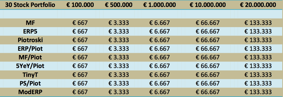
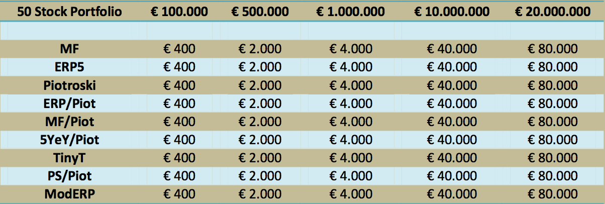
This is what the minimum daily volume limits looked like:
Minimum Daily Volume
Smallest companies excluded
They excluded companies with a market value below €15 million to make sure the companies can really be bought.
Yearly re-balancing in June each year
All portfolios were re-balanced yearly this means all companies were held for 12 months, sold and then re-invested in companies that met the requirements of the investment strategy.
Re-balancing was done in June each year. This was done because most companies in Europe have a December year end and if you re-balance in June you can be sure that year end results would have already been published and priced into the price of the stock.
The market portfolio – 250 companies excluding banks and insurance companies
The market portfolio they compared all the strategies to consisted of a weighted sum of the 250 most liquid stocks of the total industrial market of companies in the database (sorted descending by the trailing 30 days average trading volume), with weights in the proportions of the trading volume of the individual stock.
Each year, the portfolio is re-weighted based on their trading volume (based on the previous 30 days before 13/06)
They used this benchmark instead of the EUROSTOXX Index, because in this back test they wanted to include the reinvestment of dividends in the index as well as all the investment strategies tested.
To do this they included dividends by re-invested dividends by buying additional shares of the company at the closing price applicable on the ex-dividend date.
It is also important to note that the EUROSTOXX contains many banks and insurers. They were not included in the market portfolio as these companies were also not included in the back test universe.
They were excluded because these companies could not be valued with the ratios used to find investment ideas that matched the tested investment strategies.
The following chart shows how their market portfolio correlated with the EUROSTOXX index.
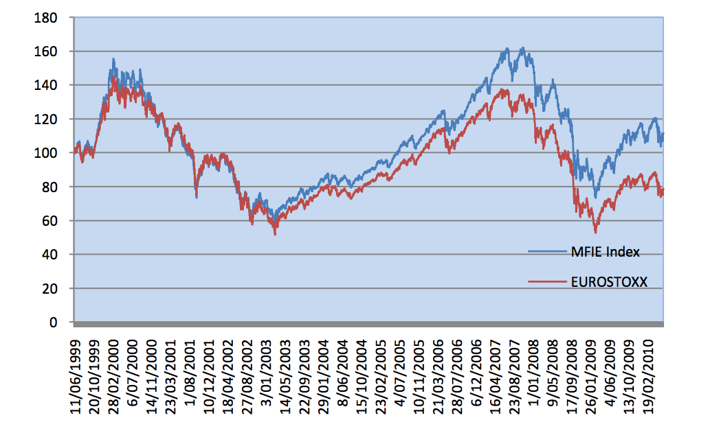
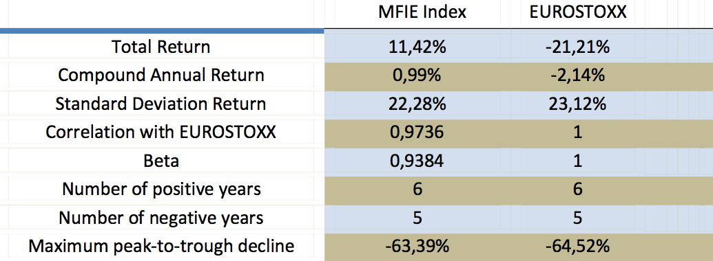
The performance difference was due to the performance of banks and insurance companies that declined substantially in the financial crisis.
Over an 11-year period (from 13/06/1999 until 13/06/2010), the Market portfolio has a total return (dividends included and reinvested) of 11.42% (or 0.99% a year) compared to -21.21% (or – 2.14 % a year) for the EUROSTOXX Index.
Looking at these numbers you can say that, over the back test period it was not good for stocks in general and that investing in bonds would have been better.
This is what they wanted to find out
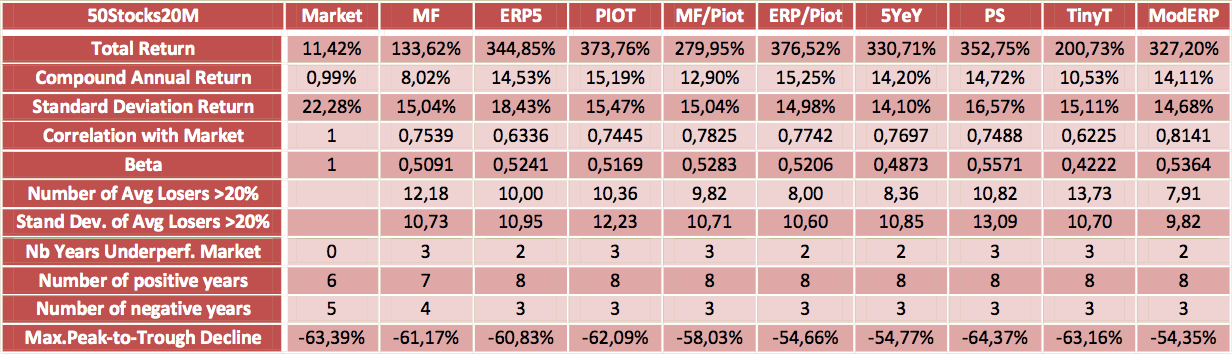
In the back test they wanted to find out:
- Average return of each value portfolio
- Standard deviation of the return
- Number of negative years of return of the different portfolios
- Number of years of underperformance against the benchmark
- Maximum Peak-to-Trough Decline (worst case return)
- Beta (volatility of the strategy compared to the market)
Academic theory states that higher-risk investments should give you higher returns over the long-term. Or in other words: the greater the risk, the greater the expected return.
But is this really true?
In his book "The new finance”, Professor Robert Haugen claims that value stocks have higher returns than growth stocks and that they are less risky!
But is this true?
In his book “Finding Alpha”, Eric Falkenstein even states that low beta stocks have higher returns. He wrote: “Nonetheless, today it is a dirty little secret, something all good quants know, but it is rarely addressed directly”
These are all the questions they wanted to answer with this research paper.
To start using Systematic Value investing in your portfolio now - Click here
How they made the back tests close to real world returns
Even though back testing is a purely theoretical exercise you can try to simulate reality by following a few rules to make sure back tested returns are as close as possible to the returns you can achieve in the real world.
This is what Philip and Luc did to make sure the tests come close to what you can earn in the real world:
1. Survival Bias:
A lot of back tests don’t include companies that went bankrupt or that were taken over. In this test, these companies were included.
2. Look ahead Bias:
When you use data for your stock ranking that was not available at the moment of portfolio formation (not yet published), your results will suffer from look-ahead bias. This bias mostly results in higher returns.
In this test they worked with accounting data from the previous fiscal year and waited 6 months to form the portfolios they tested.
Example:
For the portfolios formed in 13/6/1999, they used accounting data from the end of 1998. This made sure that all accounting data was already published when the portfolios were formed.
Portfolios were re-balanced on 13 June each year and the back tested period was from 13/06/1999 to 13/06/2010
3. Bid-Asked spread:
It is practically impossible to buy large positions in micro-cap stocks (<25 million) without moving the price up substantially.
To get around this problem in the back test they set a minimum liquidity requirement for each investment that buying and selling the positions needed to be executed in 5 working days.
They also tested that if you increased this minimum liquidity requirement by a factor 2, they did not find a significant decline in overall returns.
4. Data mining:
Back tests can be done in a number of ways. You can test thousands of different investment strategies and only publish the best results – this is called data mining. Or you can choose a few investment strategies and only test these over the back test period as they did in this research paper.
5. A Reliable Database:
They used data from Thomson DataStream as it had the best coverage of European companies.
6. Small sample Bias:
You can have a strategy that does very well over a 5-year period or longer and that may then go horribly wrong. They tested the different strategies over an 11-year period. This period was long enough to test the effectiveness of the strategies over time.
Now we come to the really exciting part of this article – what were the returns?
The Back test results - The important part
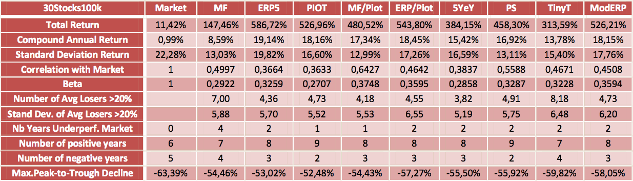
Results for the 30 company portfolios.
Starting portfolio value €100,000
Click image to enlarge
Starting portfolio value €500,000
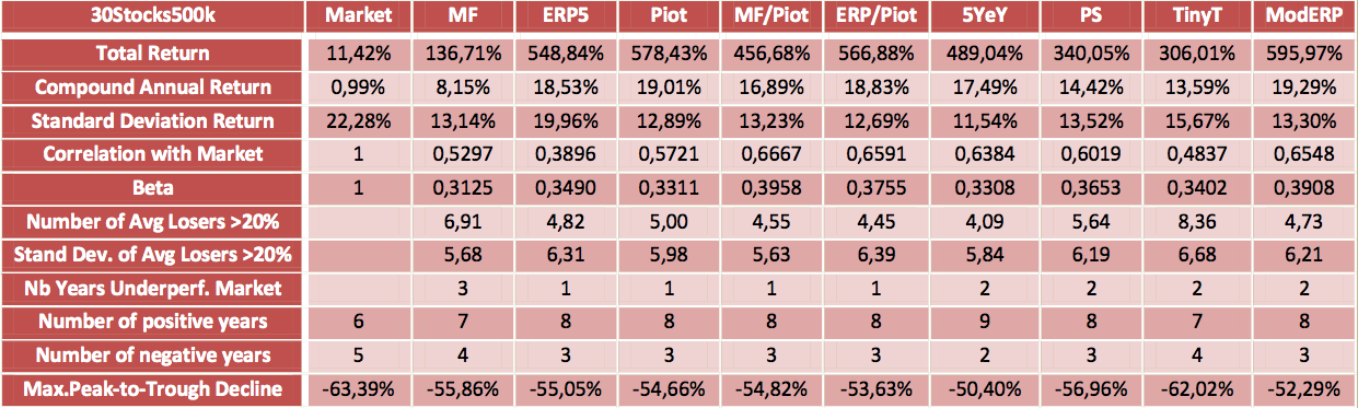
Click image to enlarge
Starting portfolio value €1 million
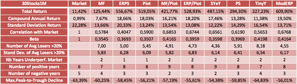
Click image to enlarge
Starting portfolio value €10 million
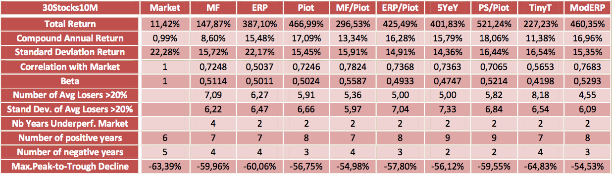
Click image to enlarge
Starting portfolio value €20 million

Click image to enlarge
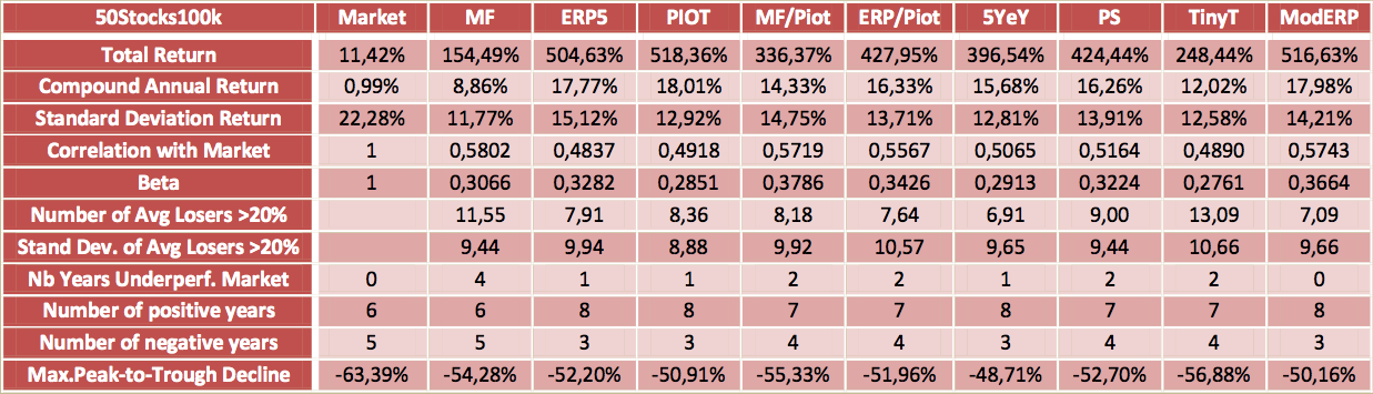
Results for the 50 company portfolios
Starting portfolio value €100,000
Click image to enlarge
Starting portfolio value €500,000

Click image to enlarge
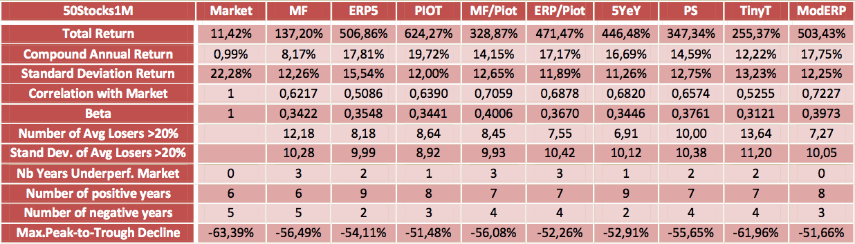
Starting portfolio value €1 million
Click image to enlarge
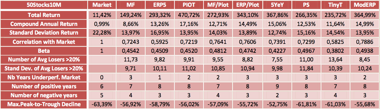
Starting portfolio value €10 million
Click image to enlarge
Starting portfolio value €20 million
Click image to enlarge
Summary
What can I learn from all the above information I am sure you are also thinking?
Below I have extracted the most important points.
The best strategy
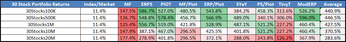
30 Stock Portfolios
Click image to enlarge
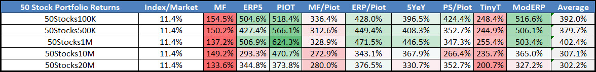
50 Stock Portfolios
Click image to enlarge
The above two tables show you the return of all the strategies for both the 30 and 50 stock portfolios.
What is interesting?
- The pure Magic Formula (MF) did not do well
- The three ERP5 strategies (ERP5, ERP/Piot, ModERP) performed great
- On average the 30 stock portfolios performed better than the 50 stock portfolios
- Returns decreased as the portfolio size (amount invested) increased
- All the strategies performed a LOT better than the market
Let’s look at the portfolio size and number of investments changes returns.
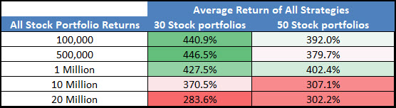
You can clearly see that the more money you have to invest the lower your returns – even though that is a nice problem to have.
Also 30 stock portfolios had higher returns than 50 stock portfolios except if you had €20 million to invest.
But never forget diversification is one of the cornerstones of safe investing, and it helps you to sleep well at night – the highest return is not the most important thing.
Conclusion
So what are the main points you can learn from all this analysis?
- Systematic value investing works – all the strategies substantially beat the market
- Smaller – 30 stock portfolios – perform better than large – 50 stock – portfolios
- More money to invest lowers your returns
- Sticking to these strategies – or even just staying invested in the market – is a lot easier than it looks – just look at the maximum declines (Maximum Peak-to-Trough Decline) of all portfolios – Never underestimate your emotions in times of extreme losses.
The tools you need to implement all of the above strategies can be found here.
It is so easy to put things off and forget, why don't you sign up right now?
To start using Systematic Value investing in your portfolio now - Click here